Dr Tom August, UKCEH
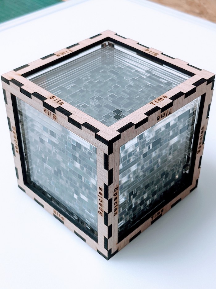
I built a physical ‘data cube’ as a way to communicate how this concept is used in biodiversity research.
Data cubes are three-dimensional arrays of data, or put another way, a stack of spreadsheets, one on top of another. In the case of my research the three dimensions of the data cube are species, location, and time. Every observation of an animal or plant in our dataset has the name of the species, where it was seen, and when it was seen, and so has a place in the three dimensional data cube. We can use these data to address a range of research questions, such as how data is distributed across sites, how species are distributed in space, and how species’ populations are changing over time.
So what stories does this physical cube tell?
First, viewed from the top we can see that as time progresses, from left to right, we see more observations (black squares), across all locations. This is real trend we see in the citizen science data that I use. This pattern is a result of wildlife reporting has become easier, through the use of smartphone apps and websites, and more and more people are getting involved in recording the wildlife that they see.

Turn the cube 90 degrees and we see how species, shown in columns below, are spread across locations, in rows. Species on the left are generalists, and so are found in most locations, but the three species on far right are specialists, only occurring in a small number of locations.

Turning the cube once more we can see how the number of observations of species changes over time. The bottom three lines are our specialists again, and you can see that over time we have fewer observations of these species. We know that habitat specialists are more sensitive to habitat change and so are often the first to experience declines.

How was it built?
I wanted the cube to tell stories, not just be random. So I generate an R script which simulated species data with specific attributes. The R code produced grids, one for each species, with rows for years and columns for locations. Each grid cell could be a 1 or 0 depending on if a species was observed in the simulation. Into the simulation I added parameters that assigned locations to habitats, gave species a habitat preference and rarity, and defined the size of the cube (I have since made a smaller version).

These were loaded into vector graphic software and prepared for a laser cutter, a machine that can very precisely move and fire a laser, following a design on a computer. The grids were cut out of Perspex, as in the image above, with a mountain of tiny black pieces cut to fill all the holes in the grid.

Finally the layers of the cube were stacked together and encased in another layer of clear Perspex, before being put inside an oak veneered frame. This frame is the only part that is glued.

The pieces took almost 3 hours to cut on the laser cutter and the black squares took two hours to place into the layers. The final piece is pretty heavy and sits on my desk at work. It has come in handy when talking about the data that we use and how we use it. Being able to hold the cube, turn it in your hands and see these different results from different angles seems to really bring the idea to life for people, whether they are new to the idea, or have been working with the concept for years.